On Friday, the CFTC posted its COT data for the first week in 2019. For crude oil, capitulation. For US Treasury bond futures, capitulation. In the latter financial market, unsurprisingly the net market position utterly collapsed during December. From a relatively high (meaning market overall short) +58k contracts that last week in November when everyone piled into liquidity hedges, the updated estimate for the week of January 8 is -8k.
Total reversal.
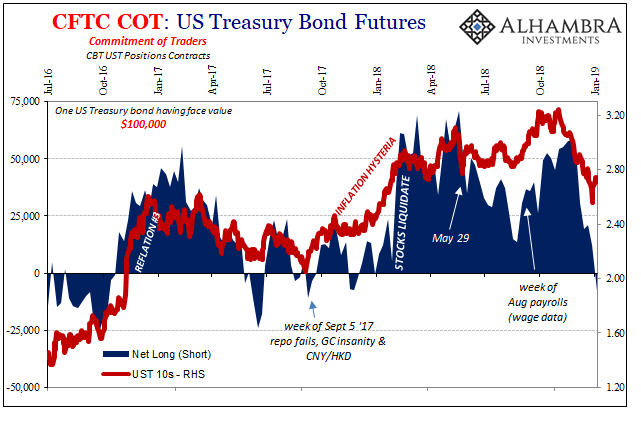
The last time we saw one of this magnitude in UST futures was in the first few months of 2014. From late December 2013 to early April 2014, the net position went from +69k to -8k; from short UST futures because interest rates have nowhere to go but up to slightly long them as liquidity hedging returned and the dollar started to do funky things. From fairy tale to prudence.
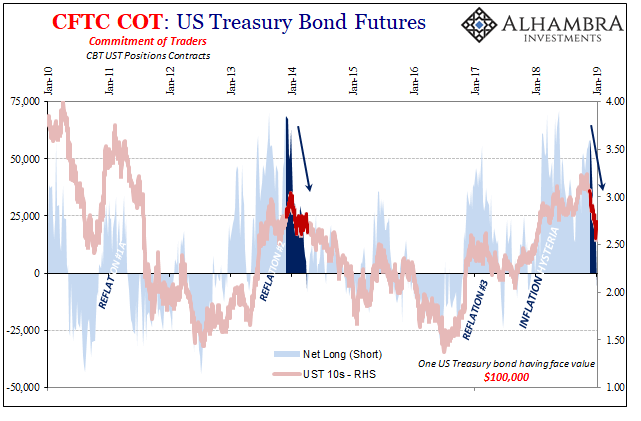
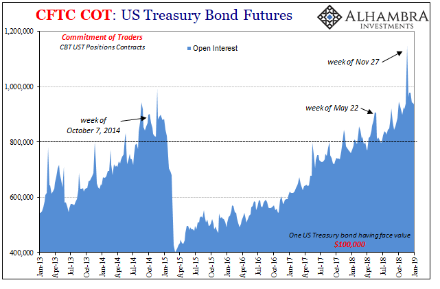
What’s unusual this time is just how quickly everything changed. In 2013-14 during the transition out of Reflation #2 and into Euro$ #3, the collapse in the market short took 17 weeks. Now as Euro$ #4 moves in, only 7 weeks.
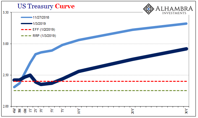
The effect on UST yields, the 10s in particular, has been largely the same regardless of time; the benchmark interest rate fell ~40 bps high to low during each shift. The primary difference is, obviously, what’s going on at the short end of the yield curve. In early 2014, QE was only starting to be tapered. To end 2018, QE is long gone and in its place are these “rate hikes.”
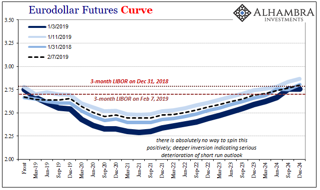
It takes something big to flip the UST curve into inversion. December 2018 and what went on absolutely qualifies – because the UST curve inverted as futures market participants capitulated. It was a paradigm change from dominant inflation expectations (thus, the market being short overall) to the more familiar deflationary sequence that starts with prominent outbreaks of liquidity hedging.
Inflation therefore accelerated growth had been rationalized repeatedly since the middle of 2017. The unemployment rate was just one factor supposedly pushing for it. Somewhat related, many proposed “money velocity” as another sea change in the global economy’s direction.
For years, money velocity as it is conventionally understood had been falling. The global economic condition during that time was disinflationary, to put it mildly, an overwhelming malaise that to central bankers required a “money printing” solution. This only contributed to falling velocities since the higher “base money” contribution didn’t immediately translate into rising (nominal) output.
This was what Dallas Fed President Richard Fisher was talking about in early 2013, what he called a head fake:
What we have done, basically, is to provide a monetary head fake. We’ve used language, which is good, and declarations, and indeed, we have, I think, had some effect.
In other words, some people were acting (stocks, in particular) on the expectation the Fed’s QE’s would amount to money printing but to that point it hadn’t actually worked out that way. Fisher, as the other FOMC members, believed the problem was timing (and Fisher was no dove, he was a thorough hawk). Eventually, all that money they printed would show up in the real economy and then the Fed would have to get aggressive.
From the perspective of January 2013, that would be a very good problem to have.
Ever since QE4, everyone has been waiting for the “money” to show up. Rising velocity would tend to suggest that it finally had, another important indication to add to the inflation/bond bear side of the ledger.
But what does the equation of exchange actually tell us? Velocity is one concept this mathematical formula introduced in a formal capacity. Economists had been talking about it ever since money was a topic to talk about. Copernicus wrote of his Monatae cudendae ratio in the early 16th century:
We in our sluggishness do not realize the dearness of everything is the result of the cheapness of money. For prices increase and decrease according to the condition of money.
John Stuart Mill and David Hume attempted to put it into quantitative terms, though realizing time was a factor (how many times money can change hands during a discrete time period). Simon Newcomb came up with the “equation of societary circulation” in 1885. Irving Fisher, borrowing heavily from Newcomb, refined it into what is now the more familiar equation of exchange: M*V = P*y (or Q, though Fisher originally presented it as T).
Like most of the rest of Economics, it is pseudo-science not science. It takes two sets of variables and makes them equal without ever having been established as so. No economist or mathematician has ever derived it from other equations that have been proven as equal. Therefore, to employ it means already that you have made the subjective choice to treat two unknown, unrelated sets as equal to each other with no evidence for the equality except past unestablished conjecture (logical fallacy).
Furthermore, on the one side, M*V, there is only one variable that can be measured balanced against a concept that may not actually be a real-world process. Again, it is assumed that velocity is real even though it cannot be in any way observed, defined, and measured as would be required for scientific precision and replicability.
Therefore, being only able to observe the one variable and by making the combination of the two variables equal to the other two variables (P*Q, or P*T, or P*y) V ends up as nothing more than confirmation bias. It is, objectively, the mathematical remainder to a series of unestablished assumptions.
If V was actually an independent and observable variable, it would not perfectly mirror M as it so often does. That’s about the only part of the equation of exchange that has been fully proven. If M changes, then V changes in the opposite direction. That’s not an explanatory equation, it is a tautology.
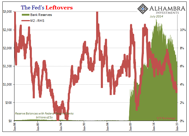
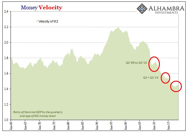
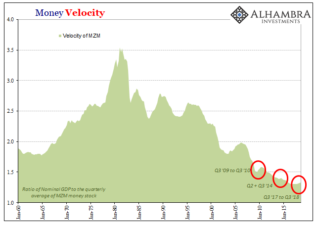
To put it in recent terms, the Fed has reduced its balance sheet and the level of bank reserves has declined. Given the equation of exchange, V necessarily has to rise again as nothing more than the remainder from a spoiled equation.
The far more interesting, and fruitful, conversation revolves around the definition of M. Bank reserves do not qualify. Economists can’t define M, and it’s a problem that has plagued the global system for more than half a century. Therefore, using something like M0 or even M2 further complicates matters by introducing a separate and even more controversial measurement problem given that FOMC officials were discussing in the early 1970’s how both numbers had already been made largely obsolete.
Or, as Alan Greenspan himself said in June 2000:
As a consequence, while of necessity it must be the case at the end of the day that inflation has to be a monetary phenomenon, a decision to base policy on measures of money presupposes that we can locate money. And that has become an increasingly dubious proposition.
If you can’t define M you have no hope of ever inferring V. Using V is a fruitless exercise in rationalizing. The results have been predictable in that way. The only requirement was, ironically, sufficient time.
The bigger problem is Fisher’s monetary head fake; everyone has been expecting the Fed’s, along with Europe’s, QE’s to start working at some point. During Euro$ #3, Chairman Yellen had cried “transitory”; as in, temporary factors were holding QE’s boost back, but once these disappeared head fake no more. This was the whole basis for 2017’s inflation hysteria.
What if, though, 2017 was just another head fake, too? December 2018.

Stay In Touch